Simple Interactive Data Analysis with Python
Posted by Chris Moffitt in articles
Interactive Python
Python is a language that allows you to create quick and simple code to do relatively complex tasks. It is very common to use the interactive python interpreter to enter a few commands in order to “figure out” how they work. If you’ve done any kind of basic python tutorial, there will be a step early in the process that asks you to type python in your command line.
The python command opens up an interpreter which allows you to type commands and get real time feedback on the results. Here is a very simple example from powerful one-liners:
$ python
Python 2.7.6 (default, Mar 22 2014, 22:59:56)
[GCC 4.8.2] on linux2
Type "help", "copyright", "credits" or "license" for more information.
>>> import pprint
>>> pprint.pprint(zip(('Byte', 'KByte', 'MByte', 'GByte', 'TByte'), (1 << 10*i for i in xrange(5))))
[('Byte', 1),
 ('KByte', 1024),
 ('MByte', 1048576),
 ('GByte', 1073741824),
 ('TByte', 1099511627776)]
>>>
While this interactive environment is really useful, it is not very conducive for more thorough exploration of python. Very early in your python journey, you’ll probably hear about IPython. IPython provides many useful features, including:
- tab completion
- object exploration
- command history
You can invoke ipython in a similar way but you’ll immediately notice a little different interface:
$ ipython
Python 2.7.6 (default, Mar 22 2014, 22:59:56)
Type "copyright", "credits" or "license" for more information.

IPython 2.3.0 -- An enhanced Interactive Python.
?         -> Introduction and overview of IPython's features.
%quickref -> Quick reference.
help      -> Python's own help system.
object?   -> Details about 'object', use 'object??' for extra details.

In [1]: import pprint

In [2]: pprint.pprint(zip(('Byte', 'KByte', 'MByte', 'GByte', 'TByte'), (1 << 10*i for i in xrange(5))))
[('Byte', 1),
 ('KByte', 1024),
 ('MByte', 1048576),
 ('GByte', 1073741824),
 ('TByte', 1099511627776)]

In [3]: help(pprint)


In [4]: pprint.
pprint.PrettyPrinter  pprint.isrecursive    pprint.pprint         pprint.warnings
pprint.isreadable     pprint.pformat        pprint.saferepr

In [4]: pprint.
In the example, I ran the same commands to get the same output but also tried the help function as well as used TAB completion after typing pprint. The other command I used was the up arrow to scroll through the history of commands, edit them and execute the results:
In [4]: pprint.pprint(zip(('Byte', 'KiloByte', 'MegaByte', 'GigaByte', 'TeraByte'), (1 << 10*i for i in xrange(5))))
[('Byte', 1),
 ('KiloByte', 1024),
 ('MegaByte', 1048576),
 ('GigaByte', 1073741824),
 ('TeraByte', 1099511627776)]

In [5]: pprint.pprint(zip(('Byte', 'KByte', 'MByte', 'GByte', 'TByte'), (1 << 10*i for i in xrange(5))))
[('Byte', 1),
 ('KByte', 1024),
 ('MByte', 1048576),
 ('GByte', 1073741824),
 ('TByte', 1099511627776)]
IPython also makes it easy to learn more about the objects you are using. If you ever get stuck, try using the ? to learn more about something:
In [9]: s = {'1','2'}

In [10]: s?
Type:        set
String form: set(['1', '2'])
Length:      2
Docstring:
set() -> new empty set object
set(iterable) -> new set object

Build an unordered collection of unique elements.

In [11]:
The functionality provided by IPython is really cool and useful and I encourage you to install it on your system and play with the various features to learn more about it.
IPython Notebook
IPython is very useful and I have used it over the years when working on Django projects. Sometime in 2011, they introduced the concept of the IPython notebook to this powerful tool. For some reason I’m late to the party but now that I’ve had the chance to use them and play with them, I can see their immense power.
The simplest way to describe an IPython Notebook is that it is a super cool way to provide the IPython console in a browser. However, it does not just provide IPython-like features in a browser, it makes it very simple to record your steps and share them with others. In the context of business applications, there are two main points to keep in mind:
- Notebooks allow you to easily interact with and explore your data
- The exploration is almost self-documenting and allows you to easily share and train others on what you are doing
Imagine you are working with Excel, and have just created a pivot table or done some other analysis. If you would like to explain to someone how to do it, what would you do? Cut and paste screen shots into Word? Record the session via some sort of screen recording tool? Hand them the Excel file and tell them to go figure it out?
None of those options are particularly good but are certainly the standard in most places where Excel rules the ad-hoc analysis world. IPython Notebooks in coordination with pandas provide a robust way to analyze large amounts of data and share your process with your teammates.
Python Data Analysis Library
The Python Data Analysis Library aka pandas is a “BSD-licensed library providing high-performance, easy-to-use data structures and data analysis tools for the Python programming language.” Pandas is a very sophisticated program and you can do some wildly complex math with it. In future articles, I’ll go through it in more detail but I wanted to do a quick sample analysis using the same data I used in my sets article.
Starting Up The Environment
Start a python notebook session:
$ ipython notebook
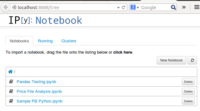
Your browser should then automatically open and redirect to the notebook server. Here is what the main screen looks like (yours will probably be empty but this shows a few example notebooks):
Clicking on the New Notebook button starts a new environment for you to code:
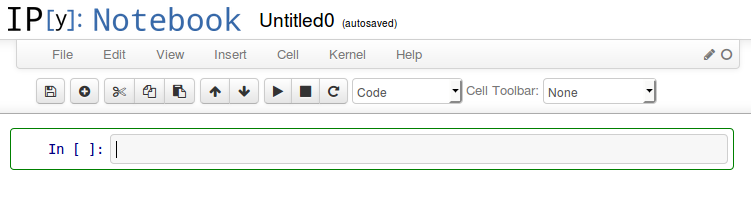
You’ll notice that the input cell looks very much like the IPython command prompt we looked at earlier.
For the rest of this article, I will show the various commands I have entered in the cells. I have chosen to download the entire session via reST so it integrates more seamlessly with my blog work flow. If people would like the actual notebook and/or data files, let me know and I’ll post them.
Additionally, the IPython Notebook has a lot of powerful features. If you’d like me to talk through it in more detail - add your input in the comments. I’m open to giving more insight into using this application.
Very Quick Data Analysis with Pandas
Now that I am up and running with my notebook, I can do some pretty powerful analysis.
First, we need to import the standard pandas libraries
import pandas as pd
import numpy as np
Next, we can read in the sample data and get a summary of how it looks.
SALES=pd.read_csv("sample-sales.csv")
SALES.head()
| Account Number | Account Name | sku | category | quantity | unit price | ext price | date | |
|---|---|---|---|---|---|---|---|---|
| 0 | 803666 | Fritsch-Glover | HX-24728 | Belt | 1 | 98.98 | 98.98 | 2014-09-28 11:56:02 |
| 1 | 64898 | O’Conner Inc | LK-02338 | Shirt | 9 | 34.80 | 313.20 | 2014-04-24 16:51:22 |
| 2 | 423621 | Beatty and Sons | ZC-07383 | Shirt | 12 | 60.24 | 722.88 | 2014-09-17 17:26:22 |
| 3 | 137865 | Gleason, Bogisich and Franecki | QS-76400 | Shirt | 5 | 15.25 | 76.25 | 2014-01-30 07:34:02 |
| 4 | 435433 | Morissette-Heathcote | RU-25060 | Shirt | 19 | 51.83 | 984.77 | 2014-08-24 06:18:12 |
Now, we can use the pivot table function to summarize the sales and turn the rows of data into something useful. We will start with something very simple
report = SALES.pivot_table(values=['quantity'],index=['Account Name'],columns=['category'], aggfunc=np.sum)
report.head(n=10)
| quantity | |||
|---|---|---|---|
| category | Belt | Shirt | Shoes |
| Account Name | |||
| Abbott PLC | NaN | NaN | 19 |
| Abbott, Rogahn and Bednar | NaN | 18 | NaN |
| Abshire LLC | NaN | 18 | 2 |
| Altenwerth, Stokes and Paucek | NaN | 13 | NaN |
| Ankunding-McCullough | NaN | 2 | NaN |
| Armstrong, Champlin and Ratke | 7 | 36 | NaN |
| Armstrong, McKenzie and Greenholt | NaN | NaN | 4 |
| Armstrong-Williamson | 19 | NaN | NaN |
| Aufderhar and Sons | NaN | NaN | 2 |
| Aufderhar-O’Hara | NaN | NaN | 11 |
This command shows us the number of products each customer purchased - all in one command! As impressive as this is, you’ll notice that there are a bunch of NaN’s in the output. This means “Not a Number” and represents places where there is no value.
Wouldn’t it be nicer if the value was a 0 instead? That’s where fill_value comes in:
report = SALES.pivot_table(values=['quantity'],index=['Account Name'],columns=['category'], fill_value=0, aggfunc=np.sum)
report.head(n=10)
| quantity | |||
|---|---|---|---|
| category | Belt | Shirt | Shoes |
| Account Name | |||
| Abbott PLC | 0 | 0 | 19 |
| Abbott, Rogahn and Bednar | 0 | 18 | 0 |
| Abshire LLC | 0 | 18 | 2 |
| Altenwerth, Stokes and Paucek | 0 | 13 | 0 |
| Ankunding-McCullough | 0 | 2 | 0 |
| Armstrong, Champlin and Ratke | 7 | 36 | 0 |
| Armstrong, McKenzie and Greenholt | 0 | 0 | 4 |
| Armstrong-Williamson | 19 | 0 | 0 |
| Aufderhar and Sons | 0 | 0 | 2 |
| Aufderhar-O’Hara | 0 | 0 | 11 |
This looks much cleaner! We will do one more thing with this example to show some of the power of the pivot_table. Let’s see how much in sales we did as well:
report = SALES.pivot_table(values=['ext price','quantity'],index=['Account Name'],columns=['category'], fill_value=0,aggfunc=np.sum)
report.head(n=10)
| ext price | quantity | |||||
|---|---|---|---|---|---|---|
| category | Belt | Shirt | Shoes | Belt | Shirt | Shoes |
| Account Name | ||||||
| Abbott PLC | 0.00 | 0.00 | 755.44 | 0 | 0 | 19 |
| Abbott, Rogahn and Bednar | 0.00 | 615.60 | 0.00 | 0 | 18 | 0 |
| Abshire LLC | 0.00 | 720.18 | 90.34 | 0 | 18 | 2 |
| Altenwerth, Stokes and Paucek | 0.00 | 843.31 | 0.00 | 0 | 13 | 0 |
| Ankunding-McCullough | 0.00 | 132.30 | 0.00 | 0 | 2 | 0 |
| Armstrong, Champlin and Ratke | 587.30 | 786.73 | 0.00 | 7 | 36 | 0 |
| Armstrong, McKenzie and Greenholt | 0.00 | 0.00 | 125.04 | 0 | 0 | 4 |
| Armstrong-Williamson | 1495.87 | 0.00 | 0.00 | 19 | 0 | 0 |
| Aufderhar and Sons | 0.00 | 0.00 | 193.54 | 0 | 0 | 2 |
| Aufderhar-O’Hara | 0.00 | 0.00 | 669.57 | 0 | 0 | 11 |
If we want, we can even output this to Excel. We have to convert it back to a DataFrame, then we can write it out to excel
report.to_excel('report.xlsx', sheet_name='Sheet1')
Showing the version of pandas in use since some syntax has changed in the more recent versions.
pd.__version__
'0.14.1'
Closing Thoughts
The purpose of this article was to give you a basic understanding of a few interactive python tools and how you can use these to do some complex analysis in a very quick and repeatable way. I plan to spend more time going through examples such as this to show how useful this toolset can be and to continue to let people know that there are alternatives to Excel when it comes to complex data analysis!
If you would like to learn more about pivot tables, please look at the Pandas Pivot Table Explained article for much more detail.
Updates
- 10-21-2014:
- Cleaned up an extra line in the Excel writing function
- Also showing the pandas version used in this example
- Added a link to the sample data
- 6-17-2015:
- Updated the excel output code
- Refer to Pandas Pivot Table Explained for a more detailed overview of pivot tables
Comments