Pandas Pivot Table Explained
Posted by Chris Moffitt in articles
Introduction
Most people likely have experience with pivot tables in Excel.
Pandas provides a similar function called (appropriately enough)
pivot_table
.
While it is exceedingly useful, I frequently find myself struggling to remember how to use the syntax
to format the output for my needs. This article will focus on explaining the pandas
pivot_table function and how to use it for your data analysis.
If you are not familiar with the concept, wikipedia explains it in high level terms. BTW, did you know that Microsoft trademarked PivotTable? Neither did I. Needless to say, I’ll be talking about a pivot table not PivotTable!
As an added bonus, I’ve created a simple cheat sheet that summarizes the pivot_table. You can find it at the end of this post and I hope it serves as a useful reference. Let me know if it is helpful.
The Data
One of the challenges with using the panda’s
pivot_table
is making sure you understand
your data and what questions you are trying to answer with the pivot table. It is a
seemingly simple function but can produce very powerful analysis very quickly.
In this scenario, I’m going to be tracking a sales pipeline (also called funnel). The basic problem is that some sales cycles are very long (think “enterprise software”, capital equipment, etc.) and management wants to understand it in more detail throughout the year.
Typical questions include:
- How much revenue is in the pipeline?
- What products are in the pipeline?
- Who has what products at what stage?
- How likely are we to close deals by year end?
Many companies will have CRM tools or other software that sales uses to track the process. While they may have useful tools for analyzing the data, inevitably someone will export the data to Excel and use a PivotTable to summarize the data.
Using a panda’s pivot table can be a good alternative because it is:
- Quicker (once it is set up)
- Self documenting (look at the code and you know what it does)
- Easy to use to generate a report or email
- More flexible because you can define custome aggregation functions
Read in the data
Let’s set up our environment first.
If you want to follow along, you can download the Excel file.
import pandas as pd
import numpy as np
Read in our sales funnel data into our DataFrame
df = pd.read_excel("../in/sales-funnel.xlsx")
df.head()
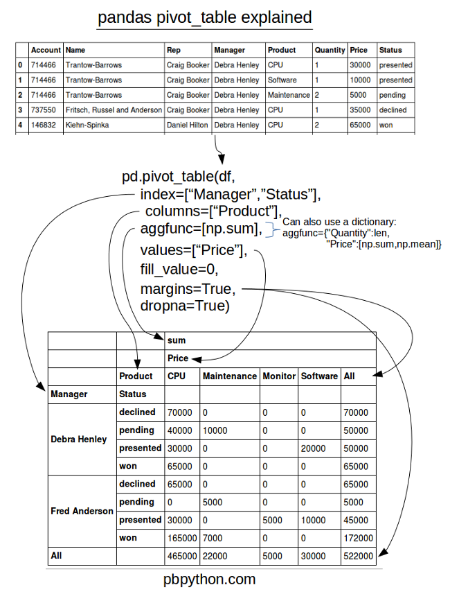
| Account | Name | Rep | Manager | Product | Quantity | Price | Status | |
|---|---|---|---|---|---|---|---|---|
| 0 | 714466 | Trantow-Barrows | Craig Booker | Debra Henley | CPU | 1 | 30000 | presented |
| 1 | 714466 | Trantow-Barrows | Craig Booker | Debra Henley | Software | 1 | 10000 | presented |
| 2 | 714466 | Trantow-Barrows | Craig Booker | Debra Henley | Maintenance | 2 | 5000 | pending |
| 3 | 737550 | Fritsch, Russel and Anderson | Craig Booker | Debra Henley | CPU | 1 | 35000 | declined |
| 4 | 146832 | Kiehn-Spinka | Daniel Hilton | Debra Henley | CPU | 2 | 65000 | won |
For convenience sake, let’s define the status column as a
category
and
set the order we want to view.
This isn’t strictly required but helps us keep the order we want as we work through analyzing the data.
df["Status"] = df["Status"].astype("category")
df["Status"].cat.set_categories(["won","pending","presented","declined"],inplace=True)
Pivot the data
As we build up the pivot table, I think it’s easiest to take it one step at a time. Add items and check each step to verify you are getting the results you expect. Don’t be afraid to play with the order and the variables to see what presentation makes the most sense for your needs.
The simplest pivot table must have a dataframe and an
index
. In this
case, let’s use the Name as our index.
pd.pivot_table(df,index=["Name"])
| Account | Price | Quantity | |
|---|---|---|---|
| Name | |||
| Barton LLC | 740150 | 35000 | 1.000000 |
| Fritsch, Russel and Anderson | 737550 | 35000 | 1.000000 |
| Herman LLC | 141962 | 65000 | 2.000000 |
| Jerde-Hilpert | 412290 | 5000 | 2.000000 |
| Kassulke, Ondricka and Metz | 307599 | 7000 | 3.000000 |
| Keeling LLC | 688981 | 100000 | 5.000000 |
| Kiehn-Spinka | 146832 | 65000 | 2.000000 |
| Koepp Ltd | 729833 | 35000 | 2.000000 |
| Kulas Inc | 218895 | 25000 | 1.500000 |
| Purdy-Kunde | 163416 | 30000 | 1.000000 |
| Stokes LLC | 239344 | 7500 | 1.000000 |
| Trantow-Barrows | 714466 | 15000 | 1.333333 |
You can have multiple indexes as well. In fact, most of the
pivot_table
args can take multiple values via a list.
pd.pivot_table(df,index=["Name","Rep","Manager"])
| Account | Price | Quantity | |||
|---|---|---|---|---|---|
| Name | Rep | Manager | |||
| Barton LLC | John Smith | Debra Henley | 740150 | 35000 | 1.000000 |
| Fritsch, Russel and Anderson | Craig Booker | Debra Henley | 737550 | 35000 | 1.000000 |
| Herman LLC | Cedric Moss | Fred Anderson | 141962 | 65000 | 2.000000 |
| Jerde-Hilpert | John Smith | Debra Henley | 412290 | 5000 | 2.000000 |
| Kassulke, Ondricka and Metz | Wendy Yule | Fred Anderson | 307599 | 7000 | 3.000000 |
| Keeling LLC | Wendy Yule | Fred Anderson | 688981 | 100000 | 5.000000 |
| Kiehn-Spinka | Daniel Hilton | Debra Henley | 146832 | 65000 | 2.000000 |
| Koepp Ltd | Wendy Yule | Fred Anderson | 729833 | 35000 | 2.000000 |
| Kulas Inc | Daniel Hilton | Debra Henley | 218895 | 25000 | 1.500000 |
| Purdy-Kunde | Cedric Moss | Fred Anderson | 163416 | 30000 | 1.000000 |
| Stokes LLC | Cedric Moss | Fred Anderson | 239344 | 7500 | 1.000000 |
| Trantow-Barrows | Craig Booker | Debra Henley | 714466 | 15000 | 1.333333 |
This is interesting but not particularly useful. What we probably want
to do is look at this by Manager and Rep. It’s easy enough to do by
changing the
index
.
pd.pivot_table(df,index=["Manager","Rep"])
| Account | Price | Quantity | ||
|---|---|---|---|---|
| Manager | Rep | |||
| Debra Henley | Craig Booker | 720237.0 | 20000.000000 | 1.250000 |
| Daniel Hilton | 194874.0 | 38333.333333 | 1.666667 | |
| John Smith | 576220.0 | 20000.000000 | 1.500000 | |
| Fred Anderson | Cedric Moss | 196016.5 | 27500.000000 | 1.250000 |
| Wendy Yule | 614061.5 | 44250.000000 | 3.000000 |
You can see that the pivot table is smart enough to start aggregating the data and summarizing it by grouping the reps with their managers. Now we start to get a glimpse of what a pivot table can do for us.
For this purpose, the Account and Quantity columns aren’t really useful.
Let’s remove it by explicitly defining the columns we care about using
the
values
field.
pd.pivot_table(df,index=["Manager","Rep"],values=["Price"])
| Price | ||
|---|---|---|
| Manager | Rep | |
| Debra Henley | Craig Booker | 20000 |
| Daniel Hilton | 38333 | |
| John Smith | 20000 | |
| Fred Anderson | Cedric Moss | 27500 |
| Wendy Yule | 44250 |
The price column automatically averages the data but we can do a count
or a sum. Adding them is simple using
aggfunc
and
np.sum
.
pd.pivot_table(df,index=["Manager","Rep"],values=["Price"],aggfunc=np.sum)
| Price | ||
|---|---|---|
| Manager | Rep | |
| Debra Henley | Craig Booker | 80000 |
| Daniel Hilton | 115000 | |
| John Smith | 40000 | |
| Fred Anderson | Cedric Moss | 110000 |
| Wendy Yule | 177000 |
aggfunc
can take a list of functions. Let’s try a mean using the numpy
mean
function and
len
to get a count.
pd.pivot_table(df,index=["Manager","Rep"],values=["Price"],aggfunc=[np.mean,len])
| mean | len | ||
|---|---|---|---|
| Price | Price | ||
| Manager | Rep | ||
| Debra Henley | Craig Booker | 20000 | 4 |
| Daniel Hilton | 38333 | 3 | |
| John Smith | 20000 | 2 | |
| Fred Anderson | Cedric Moss | 27500 | 4 |
| Wendy Yule | 44250 | 4 |
If we want to see sales broken down by the products, the
columns
variable allows us to define one or more columns.
pivot_table
is the use of
columns
and
values
.
Remember,
columns
are optional - they provide an additional way to segment the actual values you care about.
The aggregation functions are applied to the
values
you list.pd.pivot_table(df,index=["Manager","Rep"],values=["Price"],
columns=["Product"],aggfunc=[np.sum])
| sum | |||||
|---|---|---|---|---|---|
| Price | |||||
| Product | CPU | Maintenance | Monitor | Software | |
| Manager | Rep | ||||
| Debra Henley | Craig Booker | 65000 | 5000 | NaN | 10000 |
| Daniel Hilton | 105000 | NaN | NaN | 10000 | |
| John Smith | 35000 | 5000 | NaN | NaN | |
| Fred Anderson | Cedric Moss | 95000 | 5000 | NaN | 10000 |
| Wendy Yule | 165000 | 7000 | 5000 | NaN | |
The NaN’s are a bit distracting. If we want to remove them, we could use
fill_value
to set them to 0.
pd.pivot_table(df,index=["Manager","Rep"],values=["Price"],
               columns=["Product"],aggfunc=[np.sum],fill_value=0)
| sum | |||||
|---|---|---|---|---|---|
| Price | |||||
| Product | CPU | Maintenance | Monitor | Software | |
| Manager | Rep | ||||
| Debra Henley | Craig Booker | 65000 | 5000 | 0 | 10000 |
| Daniel Hilton | 105000 | 0 | 0 | 10000 | |
| John Smith | 35000 | 5000 | 0 | 0 | |
| Fred Anderson | Cedric Moss | 95000 | 5000 | 0 | 10000 |
| Wendy Yule | 165000 | 7000 | 5000 | 0 | |
I think it would be useful to add the quantity as well. Add Quantity to
the
values
list.
pd.pivot_table(df,index=["Manager","Rep"],values=["Price","Quantity"],
               columns=["Product"],aggfunc=[np.sum],fill_value=0)
| sum | |||||||||
|---|---|---|---|---|---|---|---|---|---|
| Price | Quantity | ||||||||
| Product | CPU | Maintenance | Monitor | Software | CPU | Maintenance | Monitor | Software | |
| Manager | Rep | ||||||||
| Debra Henley | Craig Booker | 65000 | 5000 | 0 | 10000 | 2 | 2 | 0 | 1 |
| Daniel Hilton | 105000 | 0 | 0 | 10000 | 4 | 0 | 0 | 1 | |
| John Smith | 35000 | 5000 | 0 | 0 | 1 | 2 | 0 | 0 | |
| Fred Anderson | Cedric Moss | 95000 | 5000 | 0 | 10000 | 3 | 1 | 0 | 1 |
| Wendy Yule | 165000 | 7000 | 5000 | 0 | 7 | 3 | 2 | 0 | |
What’s interesting is that you can move items to the index to get a
different visual representation. Remove Product from the
columns
and add to the
index
.
pd.pivot_table(df,index=["Manager","Rep","Product"],
               values=["Price","Quantity"],aggfunc=[np.sum],fill_value=0)
| sum | ||||
|---|---|---|---|---|
| Price | Quantity | |||
| Manager | Rep | Product | ||
| Debra Henley | Craig Booker | CPU | 65000 | 2 |
| Maintenance | 5000 | 2 | ||
| Software | 10000 | 1 | ||
| Daniel Hilton | CPU | 105000 | 4 | |
| Software | 10000 | 1 | ||
| John Smith | CPU | 35000 | 1 | |
| Maintenance | 5000 | 2 | ||
| Fred Anderson | Cedric Moss | CPU | 95000 | 3 |
| Maintenance | 5000 | 1 | ||
| Software | 10000 | 1 | ||
| Wendy Yule | CPU | 165000 | 7 | |
| Maintenance | 7000 | 3 | ||
| Monitor | 5000 | 2 | ||
For this data set, this representation makes more sense. Now, what if I
want to see some totals?
margins=True
does that for us.
pd.pivot_table(df,index=["Manager","Rep","Product"],
               values=["Price","Quantity"],
               aggfunc=[np.sum,np.mean],fill_value=0,margins=True)
| sum | mean | |||||
|---|---|---|---|---|---|---|
| Price | Quantity | Price | Quantity | |||
| Manager | Rep | Product | ||||
| Debra Henley | Craig Booker | CPU | 65000 | 2 | 32500.000000 | 1.000000 |
| Maintenance | 5000 | 2 | 5000.000000 | 2.000000 | ||
| Software | 10000 | 1 | 10000.000000 | 1.000000 | ||
| Daniel Hilton | CPU | 105000 | 4 | 52500.000000 | 2.000000 | |
| Software | 10000 | 1 | 10000.000000 | 1.000000 | ||
| John Smith | CPU | 35000 | 1 | 35000.000000 | 1.000000 | |
| Maintenance | 5000 | 2 | 5000.000000 | 2.000000 | ||
| Fred Anderson | Cedric Moss | CPU | 95000 | 3 | 47500.000000 | 1.500000 |
| Maintenance | 5000 | 1 | 5000.000000 | 1.000000 | ||
| Software | 10000 | 1 | 10000.000000 | 1.000000 | ||
| Wendy Yule | CPU | 165000 | 7 | 82500.000000 | 3.500000 | |
| Maintenance | 7000 | 3 | 7000.000000 | 3.000000 | ||
| Monitor | 5000 | 2 | 5000.000000 | 2.000000 | ||
| All | 522000 | 30 | 30705.882353 | 1.764706 | ||
Let’s move the analysis up a level and look at our pipeline at the manager level. Notice how the status is ordered based on our earlier category definition.
pd.pivot_table(df,index=["Manager","Status"],values=["Price"],
               aggfunc=[np.sum],fill_value=0,margins=True)
| sum | ||
|---|---|---|
| Price | ||
| Manager | Status | |
| Debra Henley | declined | 70000 |
| pending | 50000 | |
| presented | 50000 | |
| won | 65000 | |
| Fred Anderson | declined | 65000 |
| pending | 5000 | |
| presented | 45000 | |
| won | 172000 | |
| All | 522000 |
A really handy feature is the ability to pass a dictionary to the
aggfunc
so you can perform different functions on each of the values you
select. This has a side-effect of making the labels a little cleaner.
pd.pivot_table(df,index=["Manager","Status"],columns=["Product"],values=["Quantity","Price"],
               aggfunc={"Quantity":len,"Price":np.sum},fill_value=0)
| Price | Quantity | ||||||||
|---|---|---|---|---|---|---|---|---|---|
| Product | CPU | Maintenance | Monitor | Software | CPU | Maintenance | Monitor | Software | |
| Manager | Status | ||||||||
| Debra Henley | declined | 70000 | 0 | 0 | 0 | 2 | 0 | 0 | 0 |
| pending | 40000 | 10000 | 0 | 0 | 1 | 2 | 0 | 0 | |
| presented | 30000 | 0 | 0 | 20000 | 1 | 0 | 0 | 2 | |
| won | 65000 | 0 | 0 | 0 | 1 | 0 | 0 | 0 | |
| Fred Anderson | declined | 65000 | 0 | 0 | 0 | 1 | 0 | 0 | 0 |
| pending | 0 | 5000 | 0 | 0 | 0 | 1 | 0 | 0 | |
| presented | 30000 | 0 | 5000 | 10000 | 1 | 0 | 1 | 1 | |
| won | 165000 | 7000 | 0 | 0 | 2 | 1 | 0 | 0 | |
You can provide a list of aggfunctions to apply to each value too:
table = pd.pivot_table(df,index=["Manager","Status"],columns=["Product"],values=["Quantity","Price"],
               aggfunc={"Quantity":len,"Price":[np.sum,np.mean]},fill_value=0)
table
| Price | Quantity | ||||||||||||
|---|---|---|---|---|---|---|---|---|---|---|---|---|---|
| mean | sum | len | |||||||||||
| Product | CPU | Maintenance | Monitor | Software | CPU | Maintenance | Monitor | Software | CPU | Maintenance | Monitor | Software | |
| Manager | Status | ||||||||||||
| Debra Henley | declined | 35000 | 0 | 0 | 0 | 70000 | 0 | 0 | 0 | 2 | 0 | 0 | 0 |
| pending | 40000 | 5000 | 0 | 0 | 40000 | 10000 | 0 | 0 | 1 | 2 | 0 | 0 | |
| presented | 30000 | 0 | 0 | 10000 | 30000 | 0 | 0 | 20000 | 1 | 0 | 0 | 2 | |
| won | 65000 | 0 | 0 | 0 | 65000 | 0 | 0 | 0 | 1 | 0 | 0 | 0 | |
| Fred Anderson | declined | 65000 | 0 | 0 | 0 | 65000 | 0 | 0 | 0 | 1 | 0 | 0 | 0 |
| pending | 0 | 5000 | 0 | 0 | 0 | 5000 | 0 | 0 | 0 | 1 | 0 | 0 | |
| presented | 30000 | 0 | 5000 | 10000 | 30000 | 0 | 5000 | 10000 | 1 | 0 | 1 | 1 | |
| won | 82500 | 7000 | 0 | 0 | 165000 | 7000 | 0 | 0 | 2 | 1 | 0 | 0 | |
It can look daunting to try to pull this all together at one time but as
soon as you start playing with the data and slowly add the items, you
can get a feel for how it works. My general rule of thumb is that once
you use multiple
grouby
you should evaluate whether a pivot table
is a useful approach.
Advanced Pivot Table Filtering
Once you have generated your data, it is in a
DataFrame
so you can
filter on it using your standard
DataFrame
functions.
If you want to look at just one manager:
table.query('Manager == ["Debra Henley"]')
| Price | Quantity | ||||||||||||
|---|---|---|---|---|---|---|---|---|---|---|---|---|---|
| mean | sum | len | |||||||||||
| Product | CPU | Maintenance | Monitor | Software | CPU | Maintenance | Monitor | Software | CPU | Maintenance | Monitor | Software | |
| Manager | Status | ||||||||||||
| Debra Henley | declined | 35000 | 0 | 0 | 0 | 70000 | 0 | 0 | 0 | 2 | 0 | 0 | 0 |
| pending | 40000 | 5000 | 0 | 0 | 40000 | 10000 | 0 | 0 | 1 | 2 | 0 | 0 | |
| presented | 30000 | 0 | 0 | 10000 | 30000 | 0 | 0 | 20000 | 1 | 0 | 0 | 2 | |
| won | 65000 | 0 | 0 | 0 | 65000 | 0 | 0 | 0 | 1 | 0 | 0 | 0 | |
We can look at all of our pending and won deals.
table.query('Status == ["pending","won"]')
| Price | Quantity | ||||||||||||
|---|---|---|---|---|---|---|---|---|---|---|---|---|---|
| mean | sum | len | |||||||||||
| Product | CPU | Maintenance | Monitor | Software | CPU | Maintenance | Monitor | Software | CPU | Maintenance | Monitor | Software | |
| Manager | Status | ||||||||||||
| Debra Henley | pending | 40000 | 5000 | 0 | 0 | 40000 | 10000 | 0 | 0 | 1 | 2 | 0 | 0 |
| won | 65000 | 0 | 0 | 0 | 65000 | 0 | 0 | 0 | 1 | 0 | 0 | 0 | |
| Fred Anderson | pending | 0 | 5000 | 0 | 0 | 0 | 5000 | 0 | 0 | 0 | 1 | 0 | 0 |
| won | 82500 | 7000 | 0 | 0 | 165000 | 7000 | 0 | 0 | 2 | 1 | 0 | 0 | |
This a poweful feature of the
pivot_table
so do not forget that you have the full power
of pandas once you get your data into the
pivot_table
format you need.
The full notebook is available if you would like to save it as a reference.
Cheat Sheet
In order to try to summarize all of this, I have created a cheat sheet that
I hope will help you remember how to use the pandas
pivot_table
. Take a look and let me know what you think.
Thanks and good luck with creating your own pivot tables.
Comments