Monte Carlo Simulation with Python
Posted by Chris Moffitt in articles

Introduction
There are many sophisticated models people can build for solving a forecasting problem. However, they frequently stick to simple Excel models based on average historical values, intuition and some high level domain-specific heuristics. This approach may be precise enough for the problem at hand but there are alternatives that can add more information to the prediction with a reasonable amount of additional effort.
One approach that can produce a better understanding of the range of potential outcomes and help avoid the “flaw of averages” is a Monte Carlo simulation. The rest of this article will describe how to use python with pandas and numpy to build a Monte Carlo simulation to predict the range of potential values for a sales compensation budget. This approach is meant to be simple enough that it can be used for other problems you might encounter but also powerful enough to provide insights that a basic “gut-feel” model can not provide on its own.
Problem Background
For this example, we will try to predict how much money we should budget for sales commissions for the next year. This problem is useful for modeling because we have a defined formula for calculating commissions and we likely have some experience with prior years’ commissions payments.
This problem is also important from a business perspective. Sales commissions can be a large selling expense and it is important to plan appropriately for this expense. In addition, the use of a Monte Carlo simulation is a relatively simple improvement that can be made to augment what is normally an unsophisticated estimation process.
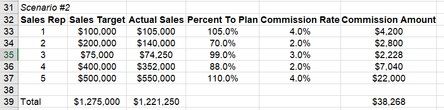
In this example, the sample sales commission would look like this for a 5 person sales force:
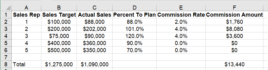
In this example, the commission is a result of this formula:
Commission Amount = Actual Sales * Commission Rate
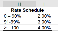
The commission rate is based on this Percent To Plan table:
Before we build a model and run the simulation, let’s look at a simple approach for predicting next year’s commission expense.
Naïve Approach to the Problem
Imagine your task as Amy or Andy analyst is to tell finance how much to budget for sales commissions for next year. One approach might be to assume everyone makes 100% of their target and earns the 4% commission rate. Plugging these values into Excel yields this:
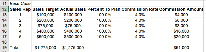
Imagine you present this to finance, and they say, “We never have everyone get the same commission rate. We need a more accurate model.”
For round two, you might try a couple of ranges:
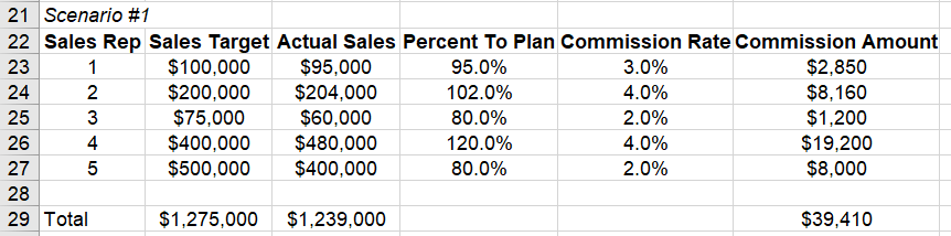
Or another one:
Now, you have a little bit more information and go back to finance. This time finance says, “this range is useful but what is your confidence in this range? Also, we need you to do this for a sales force of 500 people and model several different rates to determine the amount to budget.” Hmmm… Now, what do you do?
This simple approach illustrates the basic iterative method for a Monte Carlo simulation. You iterate through this process many times in order to determine a range of potential commission values for the year. Doing this manually by hand is challenging. Fortunately, python makes this approach much simpler.
Monte Carlo
Now that we have covered the problem at a high level, we can discuss how Monte Carlo analysis might be a useful tool for predicting commissions expenses for the next year. At its simplest level, a Monte Carlo analysis (or simulation) involves running many scenarios with different random inputs and summarizing the distribution of the results.
Using the commissions analysis, we can continue the manual process we started above but run the program 100’s or even 1000’s of times and we will get a distribution of potential commission amounts. This distribution can inform the likelihood that the expense will be within a certain window. At the end of the day, this is a prediction so we will likely never predict it exactly. We can develop a more informed idea about the potential risk of under or over budgeting.
There are two components to running a Monte Carlo simulation:
- the equation to evaluate
- the random variables for the input
We have already described the equation above. Now we need to think about how to populate the random variables.
One simple approach would be to take a random number between 0% and 200% (representing our intuition about commissions rates). However, because we pay commissions every year, we understand our problem in a little more detail and can use that prior knowledge to build a more accurate model.
Because we have paid out commissions for several years, we can look at a typical historical distribution of percent to target:
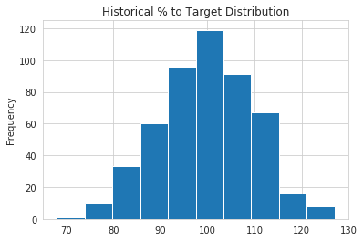
This distribution looks like a normal distribution with a mean of 100% and standard deviation of 10%. This insight is useful because we can model our input variable distribution so that it is similar to our real world experience.
If you are interested in additional details for estimating the type of distribution, I found this article interesting.
Building a Python Model
We can use pandas to construct a model that replicates the Excel spreadsheet calculation. There are other python approaches to building Monte Carlo models but I find that this pandas method is conceptually easier to comprehend if you are coming from an Excel background. It also has the added benefit of generating pandas dataframes that can be inspected and reviewed for reasonableness.
First complete our imports and set our plotting style:
import pandas as pd
import numpy as np
import seaborn as sns

sns.set_style('whitegrid')
For this model, we will use a random number generation from numpy. The handy aspect of numpy is that there are several random number generators that can create random samples based on a predefined distribution.
As described above, we know that our historical percent to target performance is centered around a a mean of 100% and standard deviation of 10%. Let’s define those variables as well as the number of sales reps and simulations we are modeling:
avg = 1
std_dev = .1
num_reps = 500
num_simulations = 1000
Now we can use numpy to generate a list of percentages that will replicate our historical normal distribution:
pct_to_target = np.random.normal(avg, std_dev, num_reps).round(2)
For this example, I have chosen to round it to 2 decimal places in order to make it very easy to see the boundaries.
Here is what the first 10 items look like:
array([0.92, 0.98, 1.1 , 0.93, 0.92, 0.99, 1.14, 1.28, 0.91, 1. ])
This is a good quick check to make sure the ranges are within expectations.
Since we are trying to make an improvement on our simple approach, we are going to stick with a normal distribution for the percent to target. By using numpy though, we can adjust and use other distribution for future models if we must. However, I do warn that you should not use other models without truly understanding them and how they apply to your situation.
There is one other value that we need to simulate and that is the actual sales target. In order to illustrate a different distribution, we are going to assume that our sales target distribution looks something like this:
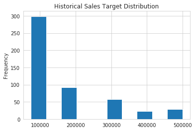
This is definitely not a normal distribution. This distribution shows us that sales targets are set into 1 of 6 buckets and the frequency gets lower as the amount increases. This distribution could be indicative of a very simple target setting process where individuals are bucketed into certain groups and given targets consistently based on their tenure, territory size or sales pipeline.
For the sake of this example, we will use a uniform distribution but assign lower probability rates for some of the values.
Here is how we can build this using
numpy.random.choice
sales_target_values = [75_000, 100_000, 200_000, 300_000, 400_000, 500_000]
sales_target_prob = [.3, .3, .2, .1, .05, .05]
sales_target = np.random.choice(sales_target_values, num_reps, p=sales_target_prob)
Admittedly this is a somewhat contrived example but I wanted to show how different distributions could be incorporated into our model.
Now that we know how to create our two input distributions, let’s build up a pandas dataframe:
df = pd.DataFrame(index=range(num_reps), data={'Pct_To_Target': pct_to_target,
                                               'Sales_Target': sales_target})

df['Sales'] = df['Pct_To_Target'] * df['Sales_Target']
Here is what our new dataframe looks like:
| Pct_To_Target | Sales_Target | Sales | |
|---|---|---|---|
| 0 | 0.92 | 100000 | 92000.0 |
| 1 | 0.98 | 75000 | 73500.0 |
| 2 | 1.10 | 500000 | 550000.0 |
| 3 | 0.93 | 200000 | 186000.0 |
| 4 | 0.92 | 300000 | 276000.0 |
You might notice that I did a little trick to calculate the actual sales amount. For this problem, the actual sales amount may change greatly over the years but the performance distribution remains remarkably consistent. Therefore, I’m using the random distributions to generate my inputs and backing into the actual sales.
The final piece of code we need to create is a way to map our
Pct_To_Target
to the commission rate. Here is the function:
def calc_commission_rate(x):
    """ Return the commission rate based on the table:
    0-90% = 2%
    91-99% = 3%
    >= 100 = 4%
    """
    if x <= .90:
        return .02
    if x <= .99:
        return .03
    else:
        return .04
The added benefit of using python instead of Excel is that we can create much more complex logic that is easier to understand than if we tried to build a complex nested if statement in Excel.
Now we create our commission rate and multiply it times sales:
df['Commission_Rate'] = df['Pct_To_Target'].apply(calc_commission_rate)
df['Commission_Amount'] = df['Commission_Rate'] * df['Sales']
Which yields this result, which looks very much like an Excel model we might build:
| Pct_To_Target | Sales_Target | Sales | Commission_Rate | Commission_Amount | |
|---|---|---|---|---|---|
| 0 | 97.0 | 100000 | 97000.0 | .03 | 2910.0 |
| 1 | 92.0 | 400000 | 368000.0 | .03 | 11040.0 |
| 2 | 97.0 | 200000 | 194000.0 | .03 | 5820.0 |
| 3 | 103.0 | 200000 | 206000.0 | .04 | 8240.0 |
| 4 | 87.0 | 75000 | 65250.0 | .02 | 1305.0 |
There you have it!
We have replicated a model that is similar to what we would have done in Excel but we used some more sophisticated distributions than just throwing a bunch of random number inputs into the problem.
If we sum up the values (only the top 5 are shown above) in the
Commission_Amount
column, we can see that this simulation shows that we would pay $2,923,100.
Let’s Loop
The real “magic” of the Monte Carlo simulation is that if we run a simulation
many times, we start to develop a picture of the likely distribution of results.
In Excel, you would need VBA or another plugin to run multiple iterations. In
python, we can use a
for
loop to run as many simulations as we’d like.
In addition to running each simulation, we save the results we care about in a list that we will turn into a dataframe for further analysis of the distribution of results.
Here is the full for loop code:
# Define a list to keep all the results from each simulation that we want to analyze
all_stats = []

# Loop through many simulations
for i in range(num_simulations):

    # Choose random inputs for the sales targets and percent to target
    sales_target = np.random.choice(sales_target_values, num_reps, p=sales_target_prob)
    pct_to_target = np.random.normal(avg, std_dev, num_reps).round(2)

    # Build the dataframe based on the inputs and number of reps
    df = pd.DataFrame(index=range(num_reps), data={'Pct_To_Target': pct_to_target,
                                                   'Sales_Target': sales_target})

    # Back into the sales number using the percent to target rate
    df['Sales'] = df['Pct_To_Target'] * df['Sales_Target']

    # Determine the commissions rate and calculate it
    df['Commission_Rate'] = df['Pct_To_Target'].apply(calc_commission_rate)
    df['Commission_Amount'] = df['Commission_Rate'] * df['Sales']

    # We want to track sales,commission amounts and sales targets over all the simulations
    all_stats.append([df['Sales'].sum().round(0),
                      df['Commission_Amount'].sum().round(0),
                      df['Sales_Target'].sum().round(0)])
While this may seem a little intimidating at first, we are only including 7 python statements inside this loop that we can run as many times as we want. On my standard laptop, I can run 1000 simulations in 2.75s so there is no reason I can’t do this many more times if need be.
At some point, there are diminishing returns. The results of 1 Million simulations are not necessarily any more useful than 10,000. My advice is to try different amounts and see how the output changes.
In order to analyze the results of the simulation, I will build a dataframe
from
all_stats
:
results_df = pd.DataFrame.from_records(all_stats, columns=['Sales',
                                                           'Commission_Amount',
                                                           'Sales_Target'])
Now, it is easy to see what the range of results look like:
results_df.describe().style.format('{:,}')
| Sales | Commission_Amount | Sales_Target | |
|---|---|---|---|
| count | 1,000.0 | 1,000.0 | 1,000.0 |
| mean | 83,617,936.0 | 2,854,916.1 | 83,619,700.0 |
| std | 2,727,222.9 | 103,003.9 | 2,702,621.8 |
| min | 74,974,750.0 | 2,533,810.0 | 75,275,000.0 |
| 25% | 81,918,375.0 | 2,786,088.0 | 81,900,000.0 |
| 50% | 83,432,500 | 2,852,165.0 | 83,525,000.0 |
| 75% | 85,318,440.0 | 2,924,053.0 | 85,400,000.0 |
| max | 92,742,500.0 | 3,214,385.0 | 91,925,000.0 |
Graphically, it looks like this:
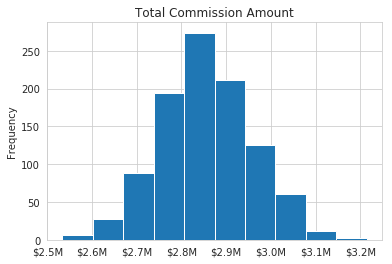
So, what does this chart and the output of describe tell us? We can see that the average commissions expense is $2.85M and the standard deviation is $103K. We can also see that the commissions payment can be as low as $2.5M or as high as $3.2M.
Based on these results, how comfortable are you that the expense for commissions will be less than $3M? Or, if someone says, “Let’s only budget $2.7M” would you feel comfortable that your expenses would be below that amount? Probably not.
Therein lies one of the benefits of the Monte Carlo simulation. You develop a better understanding of the distribution of likely outcomes and can use that knowledge plus your business acumen to make an informed estimate.
The other value of this model is that you can model many different assumptions and see what happens. Here are some simple changes you can make to see how the results change:
- Increase top commission rate to 5%
- Decrease the number of sales people
- Change the expected standard deviation to a higher amount
- Modify the distribution of targets
Now that the model is created, making these changes is as simple as a few variable tweaks and re-running your code. You can view the notebook associated with this post on github.
Another observation about Monte Carlo simulations is that they are relatively easy to explain to the end user of the prediction. The person receiving this estimate may not have a deep mathematical background but can intuitively understand what this simulation is doing and how to assess the likelihood of the range of potential results.
Finally, I think the approach shown here with python is easier to understand and replicate than some of the Excel solutions you may encounter. Because python is a programming language, there is a linear flow to the calculations which you can follow.
Conclusion
A Monte Carlo simulation is a useful tool for predicting future results by calculating a formula multiple times with different random inputs. This is a process you can execute in Excel but it is not simple to do without some VBA or potentially expensive third party plugins. Using numpy and pandas to build a model and generate multiple potential results and analyze them is relatively straightforward. The other added benefit is that analysts can run many scenarios by changing the inputs and can move on to much more sophisticated models in the future if the needs arise. Finally, the results can be shared with non-technical users and facilitate discussions around the uncertainty of the final results.
I hope this example is useful to you and gives you ideas that you can apply to your own problems. Please feel free to leave a comment if you find this article helpful for developing your own estimation models.
Updates
- 19-March-2019: Based on comments from reddit, I have made another implementation which is faster.
Comments