Understanding the Transform Function in Pandas
Posted by Chris Moffitt in articles
Introduction
One of the compelling features of pandas is that it has a rich library of methods for manipulating
data. However, there are times when it is not clear what the various functions
do and how to use them. If you are approaching a problem from an Excel mindset,
it can be difficult to translate the planned solution into the unfamiliar pandas command.
One of those “unknown” functions is the
transform
method.
Even after using pandas for a while, I have never had the chance to use this function
so I recently took some time to figure out what it is and how it could be helpful
for real world analysis. This article will walk through an example where
transform
can be used to efficiently summarize data.
What is transform?
I have found the best coverage of this topic in Jake VanderPlas’ excellent Python Data Science Handbook. I plan to write a review on this book in the future but the short and sweet is that it is a great resource that I highly recommend.
As described in the book,
transform
is an operation used in conjunction
with
groupby
(which is one of the most useful operations in pandas). I
suspect most pandas users likely have used
aggregate
,
filter
or
apply
with
groupby
to summarize data. However,
transform
is a little more difficult to understand - especially coming from an Excel world.
Since Jake made all of his book available via jupyter notebooks it is a good place
to start to understand how transform is unique:
While aggregation must return a reduced version of the data, transformation can return some transformed version of the full data to recombine. For such a transformation, the output is the same shape as the input. A common example is to center the data by subtracting the group-wise mean.
With that basic definition, I will go through another example that can explain how this is useful in other instances outside of centering data.
Problem Set
For this example, we will analyze some fictitious sales data. In order to keep the dataset small, here is a sample of 12 sales transactions for our company:
| account | name | order | sku | quantity | unit price | ext price | |
|---|---|---|---|---|---|---|---|
| 0 | 383080 | Will LLC | 10001 | B1-20000 | 7 | 33.69 | 235.83 |
| 1 | 383080 | Will LLC | 10001 | S1-27722 | 11 | 21.12 | 232.32 |
| 2 | 383080 | Will LLC | 10001 | B1-86481 | 3 | 35.99 | 107.97 |
| 3 | 412290 | Jerde-Hilpert | 10005 | S1-06532 | 48 | 55.82 | 2679.36 |
| 4 | 412290 | Jerde-Hilpert | 10005 | S1-82801 | 21 | 13.62 | 286.02 |
| 5 | 412290 | Jerde-Hilpert | 10005 | S1-06532 | 9 | 92.55 | 832.95 |
| 6 | 412290 | Jerde-Hilpert | 10005 | S1-47412 | 44 | 78.91 | 3472.04 |
| 7 | 412290 | Jerde-Hilpert | 10005 | S1-27722 | 36 | 25.42 | 915.12 |
| 8 | 218895 | Kulas Inc | 10006 | S1-27722 | 32 | 95.66 | 3061.12 |
| 9 | 218895 | Kulas Inc | 10006 | B1-33087 | 23 | 22.55 | 518.65 |
| 10 | 218895 | Kulas Inc | 10006 | B1-33364 | 3 | 72.30 | 216.90 |
| 11 | 218895 | Kulas Inc | 10006 | B1-20000 | -1 | 72.18 | -72.18 |
You can see in the data that the file contains 3 different orders (10001, 10005 and 10006) and that each order consists has multiple products (aka skus).
The question we would like to answer is: “What percentage of the order total does each sku represent?”
For example, if we look at order 10001 with a total of $576.12, the break down would be:
- B1-20000 = $235.83 or 40.9%
- S1-27722 = $232.32 or 40.3%
- B1-86481 = $107.97 or 18.7%
The tricky part in this calculation is that we need to get a total for each order and combine it back with the transaction level detail in order to get the percentages. In Excel, you could try to use some version of a subtotal to try to calculate the values.
First Approach - Merging
If you are familiar with pandas, your first inclination is going to be trying to group the data into a new dataframe and combine it in a multi-step process. Here’s what that approach would look like.
Import all the modules we need and read in our data:
import pandas as pd

df = pd.read_excel("sales_transactions.xlsx")
Now that the data is in a dataframe, determining the total by order is simple with the
help of the standard
groupby
aggregation.
df.groupby('order')["ext price"].sum()
order
10001     576.12
10005    8185.49
10006    3724.49
Name: ext price, dtype: float64
Here is a simple image showing what is happening with the standard
groupby
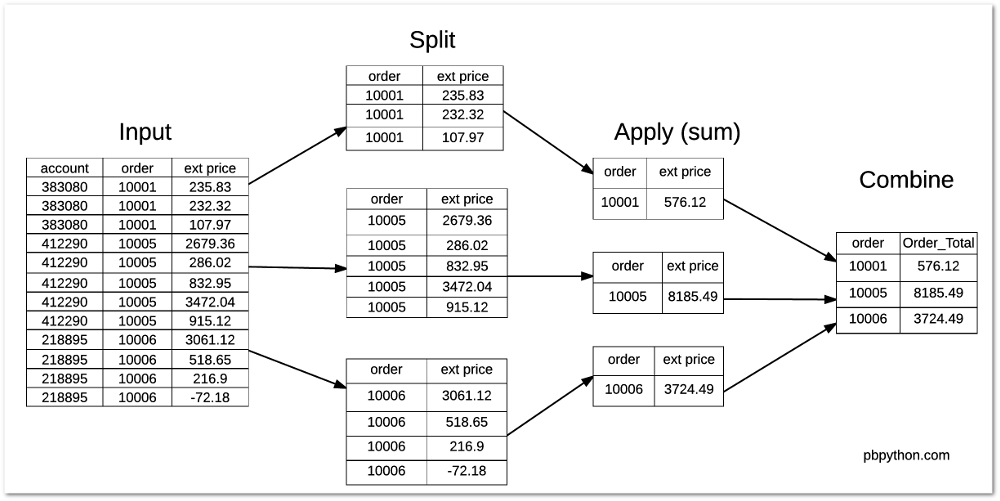
The tricky part is figuring out how to combine this data back with the original dataframe. The first instinct is to create a new dataframe with the totals by order and merge it back with the original. We could do something like this:
order_total = df.groupby('order')["ext price"].sum().rename("Order_Total").reset_index()
df_1 = df.merge(order_total)
df_1["Percent_of_Order"] = df_1["ext price"] / df_1["Order_Total"]
| account | name | order | sku | quantity | unit price | ext price | order total | Order_Total | Percent_of_Order | |
|---|---|---|---|---|---|---|---|---|---|---|
| 0 | 383080 | Will LLC | 10001 | B1-20000 | 7 | 33.69 | 235.83 | 576.12 | 576.12 | 0.409342 |
| 1 | 383080 | Will LLC | 10001 | S1-27722 | 11 | 21.12 | 232.32 | 576.12 | 576.12 | 0.403249 |
| 2 | 383080 | Will LLC | 10001 | B1-86481 | 3 | 35.99 | 107.97 | 576.12 | 576.12 | 0.187409 |
| 3 | 412290 | Jerde-Hilpert | 10005 | S1-06532 | 48 | 55.82 | 2679.36 | 8185.49 | 8185.49 | 0.327330 |
| 4 | 412290 | Jerde-Hilpert | 10005 | S1-82801 | 21 | 13.62 | 286.02 | 8185.49 | 8185.49 | 0.034942 |
| 5 | 412290 | Jerde-Hilpert | 10005 | S1-06532 | 9 | 92.55 | 832.95 | 8185.49 | 8185.49 | 0.101759 |
| 6 | 412290 | Jerde-Hilpert | 10005 | S1-47412 | 44 | 78.91 | 3472.04 | 8185.49 | 8185.49 | 0.424170 |
| 7 | 412290 | Jerde-Hilpert | 10005 | S1-27722 | 36 | 25.42 | 915.12 | 8185.49 | 8185.49 | 0.111798 |
| 8 | 218895 | Kulas Inc | 10006 | S1-27722 | 32 | 95.66 | 3061.12 | 3724.49 | 3724.49 | 0.821890 |
| 9 | 218895 | Kulas Inc | 10006 | B1-33087 | 23 | 22.55 | 518.65 | 3724.49 | 3724.49 | 0.139254 |
| 10 | 218895 | Kulas Inc | 10006 | B1-33364 | 3 | 72.30 | 216.90 | 3724.49 | 3724.49 | 0.058236 |
| 11 | 218895 | Kulas Inc | 10006 | B1-20000 | -1 | 72.18 | -72.18 | 3724.49 | 3724.49 | -0.019380 |
This certainly works but there are several steps needed to get the data combined in the manner we need.
Second Approach - Using Transform
Using the original data, let’s try using
transform
and
groupby
and
see what we get:
df.groupby('order')["ext price"].transform('sum')
0      576.12
1      576.12
2      576.12
3     8185.49
4     8185.49
5     8185.49
6     8185.49
7     8185.49
8     3724.49
9     3724.49
10    3724.49
11    3724.49
dtype: float64
You will notice how this returns a different size data set from our normal
groupby
functions. Instead of only showing the totals for 3 orders, we retain the same number
of items as the original data set. That is the unique feature of using
transform
.
The final step is pretty simple:
df["Order_Total"] = df.groupby('order')["ext price"].transform('sum')
df["Percent_of_Order"] = df["ext price"] / df["Order_Total"]
| account | name | order | sku | quantity | unit price | ext price | order total | Order_Total | Percent_of_Order | |
|---|---|---|---|---|---|---|---|---|---|---|
| 0 | 383080 | Will LLC | 10001 | B1-20000 | 7 | 33.69 | 235.83 | 576.12 | 576.12 | 0.409342 |
| 1 | 383080 | Will LLC | 10001 | S1-27722 | 11 | 21.12 | 232.32 | 576.12 | 576.12 | 0.403249 |
| 2 | 383080 | Will LLC | 10001 | B1-86481 | 3 | 35.99 | 107.97 | 576.12 | 576.12 | 0.187409 |
| 3 | 412290 | Jerde-Hilpert | 10005 | S1-06532 | 48 | 55.82 | 2679.36 | 8185.49 | 8185.49 | 0.327330 |
| 4 | 412290 | Jerde-Hilpert | 10005 | S1-82801 | 21 | 13.62 | 286.02 | 8185.49 | 8185.49 | 0.034942 |
| 5 | 412290 | Jerde-Hilpert | 10005 | S1-06532 | 9 | 92.55 | 832.95 | 8185.49 | 8185.49 | 0.101759 |
| 6 | 412290 | Jerde-Hilpert | 10005 | S1-47412 | 44 | 78.91 | 3472.04 | 8185.49 | 8185.49 | 0.424170 |
| 7 | 412290 | Jerde-Hilpert | 10005 | S1-27722 | 36 | 25.42 | 915.12 | 8185.49 | 8185.49 | 0.111798 |
| 8 | 218895 | Kulas Inc | 10006 | S1-27722 | 32 | 95.66 | 3061.12 | 3724.49 | 3724.49 | 0.821890 |
| 9 | 218895 | Kulas Inc | 10006 | B1-33087 | 23 | 22.55 | 518.65 | 3724.49 | 3724.49 | 0.139254 |
| 10 | 218895 | Kulas Inc | 10006 | B1-33364 | 3 | 72.30 | 216.90 | 3724.49 | 3724.49 | 0.058236 |
| 11 | 218895 | Kulas Inc | 10006 | B1-20000 | -1 | 72.18 | -72.18 | 3724.49 | 3724.49 | -0.019380 |
As an added bonus, you could combine into one statement if you did not want to show the individual order totals:
df["Percent_of_Order"] = df["ext price"] / df.groupby('order')["ext price"].transform('sum')
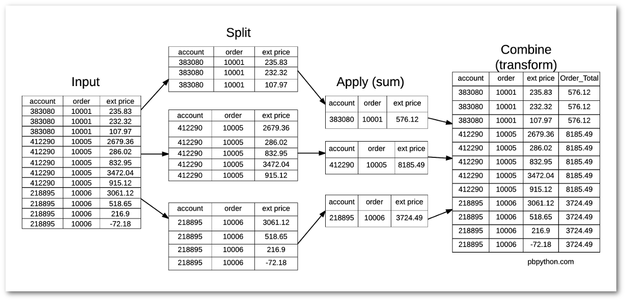
Here is a diagram to show what is happening:
After taking the time to understand
transform
, I think you will agree that this
tool can be very powerful - even if it is a unique approach as compared to the
standard Excel mindset.
Conclusion
I am continually amazed at the power of pandas to make complex numerical manipulations
very efficient. Despite working with pandas for a while, I never took the time to figure
out how to use
transform.
Now that I understand how it works, I am sure
I will be able to use it in future analysis and hope that you will find this useful
as well.
Comments